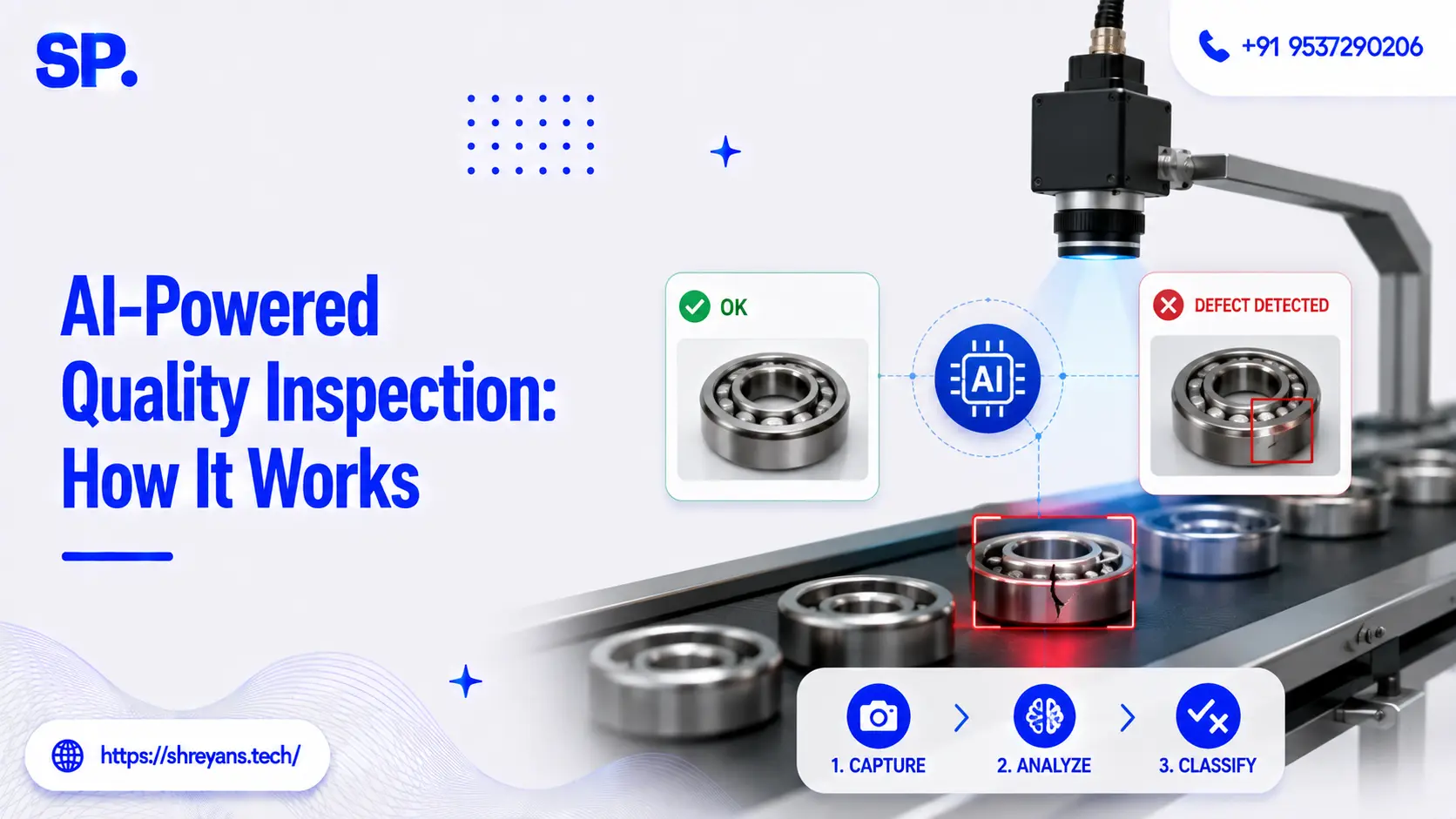
AI-Powered Quality Inspection: How It Works

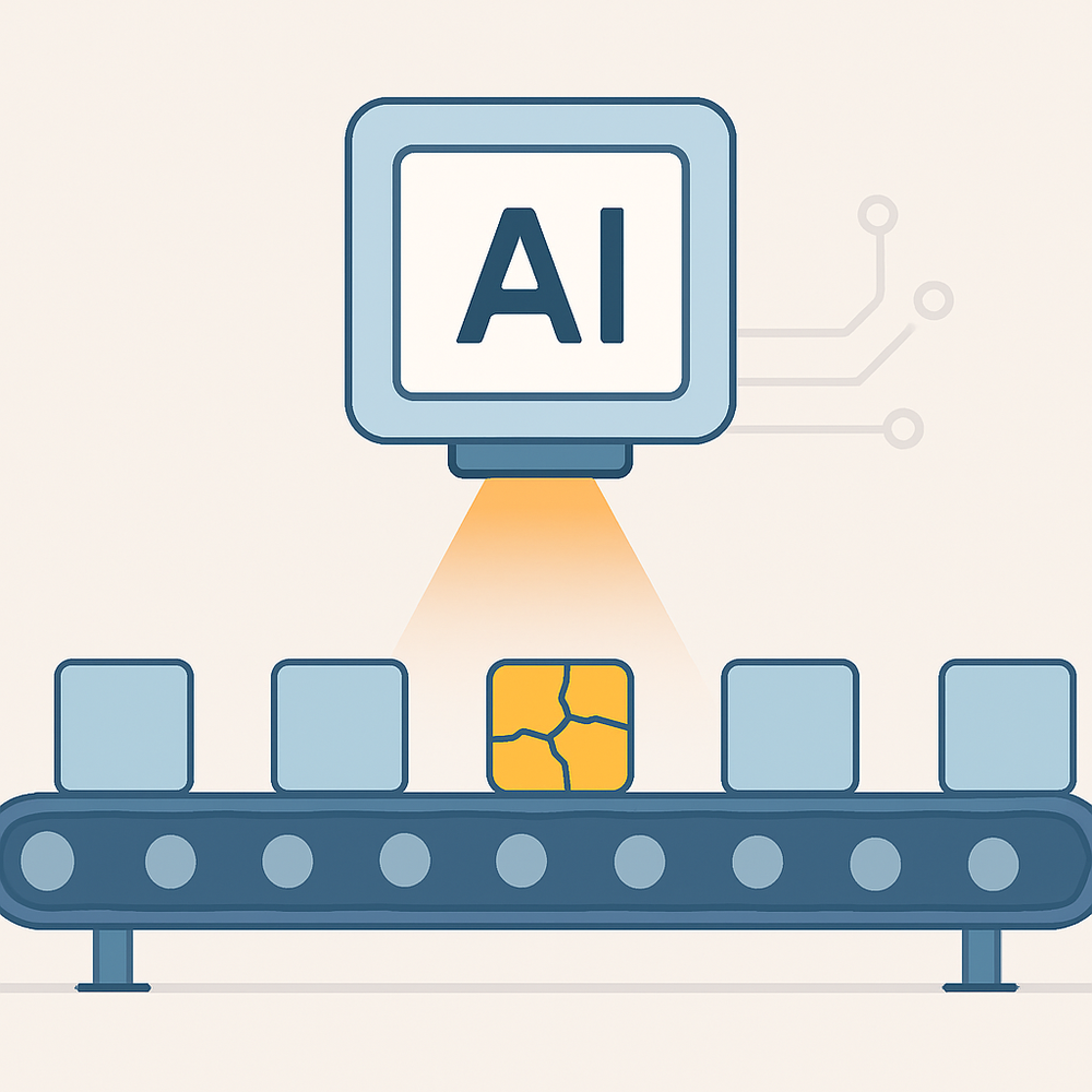
A healthy production line has a data problem hiding inside it. For every defective part it produces, it produces thousands of good ones. That imbalance breaks the most obvious approach to teaching a model what a defect looks like, because there simply aren't enough examples of each defect type to learn from.

The solution that modern ai quality inspection systems use is counterintuitive: train the model only on good parts, and let it flag anything that doesn't match. Understanding why that works, and what sits around it, is the difference between a system that catches the defect nobody anticipated and one that waves it straight through.

Strip away the vendor language and every deployment runs the same four steps on every part that passes the camera.

None of this runs on its own. A line-control layer, a PLC, SCADA system, robot controller, or conveyor controller, triggers the camera at the right moment, controls the lighting, assigns each image to the correct product identifier, and activates the reject or rework mechanism when the model calls a fail. computer vision in manufacturing covers how these systems sit within broader production and quality workflows.

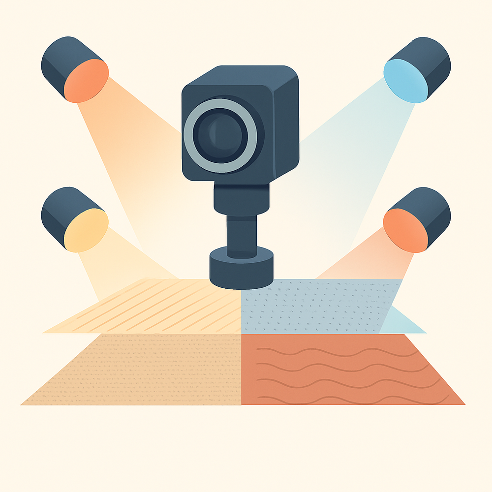
The least glamorous part of a vision system is the part most likely to determine whether it works. If lighting varies between the images the model trained on and the images it sees in production, accuracy collapses regardless of how good the model is, because the model is comparing against a normal it no longer recognises.

Different defects need different illumination. Coaxial lighting, where light travels along the same axis as the camera, produces uniform illumination without shadows and suits flat reflective surfaces. Angled or grazing light makes surface scratches and dents visible by casting shadows into them. Backlighting reveals dimensional and edge defects as silhouettes. Sub-surface problems, casting porosity, weld porosity, composite voids, need specialised lighting or entirely different sensing altogether.

This is why a system that performs well in a vendor demo can fail on your line. The demo controlled the lighting; your factory floor may not, and ambient light from a window or a seasonal change in overhead lighting is enough to shift results.

This is the core technical decision, and it follows directly from the class imbalance in the opening.

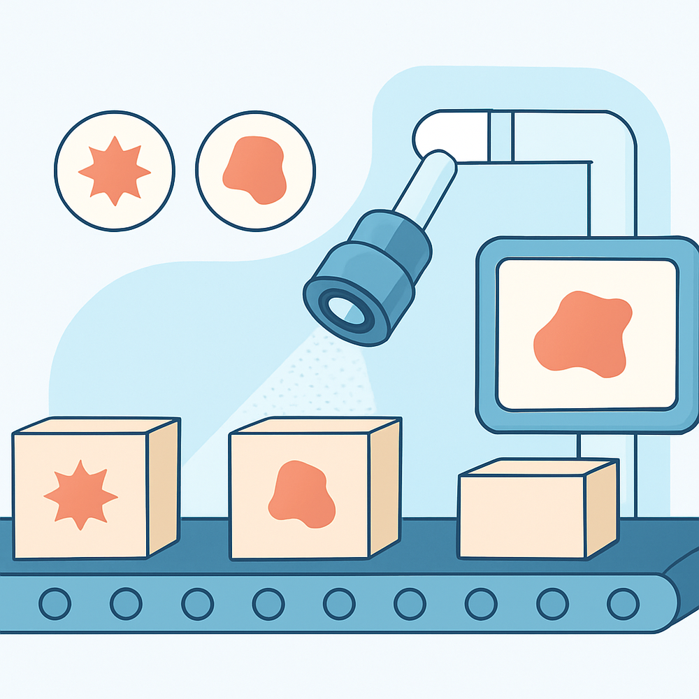
The output is richer than a binary pass or fail. Depending on the model family, a system returns a defect class, a bounding box locating the defect, a pixel-level segmentation mask outlining its exact shape, and a confidence score for the judgement.

Those outputs feed severity-ranked thresholds that decide what physically happens: pass, divert to rework, reject outright, or stop the line. Setting those thresholds is a business decision rather than a technical one, because it's really a choice about the relative cost of a false reject, throwing away a good part, versus a false accept, shipping a defective one. A safety-critical component and a cosmetic panel warrant very different settings, and real-world CV projects illustrates how differently this plays out across domains.

Inference itself typically runs on an edge GPU near the line rather than in the cloud, because a conveyor moving at production speed can't wait on a network round trip, and many plants won't route production imagery off-site regardless.

A vision model degrades over time. Camera position drifts fractionally, lighting ages, suppliers change material finish, and new product variants appear. Without a maintenance loop, accuracy declines quietly, and the failure is invisible until someone audits rejected parts.

The standard mechanism is an active learning loop. When the model encounters something it flags with low confidence, the system captures the image and routes it to an operator for review. Once the operator confirms whether it was a genuine defect, that image joins the training dataset, and retraining runs in the background without interrupting production.

The 2026 research direction worth knowing about is on-device continual learning for high-mix environments, where product variants change frequently and cloud retraining is too slow. Published work extending PatchCore with incremental updates reports a 12% accuracy improvement over batch retraining baselines alongside an 80% reduction in memory use, making it practical on the legacy edge hardware most plants actually have rather than requiring new infrastructure.