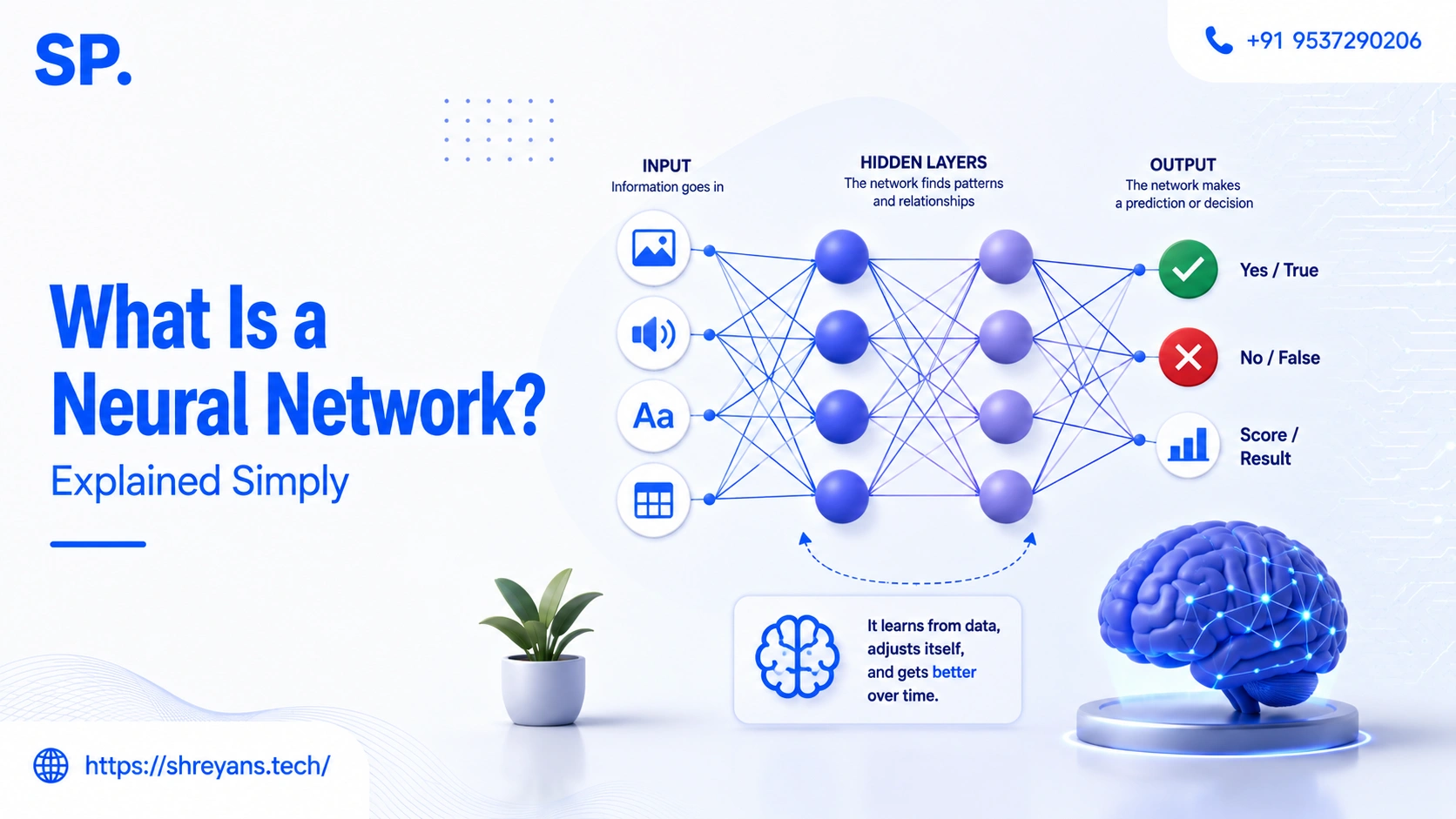
According to DemandSage statistics, around ninety percent of businesses adopt artificial intelligence solutions to stay competitive, and seventy-seven percent of devices already include AI features. The global neural network software market is projected to reach forty-five point six three billion US dollars in 2026, growing at a thirty-one point two five percent compound annual growth rate through 2031. These figures reflect the rapid expansion of AI capabilities that were impractical just a decade ago.
In January 2026, the UK government's AI Growth Zones policy highlighted increasing data centre demand and capacity challenges, with regulators focusing on reducing planning barriers and accelerating grid connections to support the AI infrastructure boom. Meanwhile, IBM's Cost of a Data Breach Report 2026 revealed a fifty-six percent increase in AI-driven attacks, demonstrating how neural networks power both defensive and offensive cybersecurity operations in equal measure. The report documented average breach costs rising to 5.35 million US dollars, with AI-enabled incidents taking longer to contain due to their sophisticated nature.
The Basic Building Block: Artificial Neurons
Every neural network is just a collection of neurons, each making tiny mathematical decisions. My goal today is going to be to show you what a single neuron does, and how it transforms numbers into signals and learns which features within its training data matter most. The neuron operates through weighted connections that amplify or dampen incoming signals, followed by an activation function that determines whether the neuron should fire based on a threshold or learned condition.
The mathematical foundation begins with a simple linear combination: each input value multiplies a corresponding weight, and these products sum together with a bias term. This weighted sum represents the neuron's raw activation level before any non-linear transformation. The bias acts as a baseline threshold, allowing the neuron to activate even when all inputs are zero, which provides essential flexibility in network architecture. In ResNet-50, for example, each residual block contains neurons that learn identity mappings through skip connections, enabling the network to train effectively with fifty-three layers by allowing gradients to flow directly through the skip pathways during backpropagation.
How Neurons Process Inputs
The processing operation follows the equation: output = activation_function(weight1*input1 + weight2*input2 + ... + bias). This linear transformation alone would make neural networks equivalent to simple linear models, incapable of learning complex patterns. The weights determine the importance of each input feature, and during training, backpropagation adjusts these values to minimise prediction error through gradient descent optimisation.
Activation Functions in Practice
Non-linear activation functions like ReLU (Rectified Linear Unit) enable neural networks to approximate any continuous function, a capability known as universal approximation. ReLU outputs the input directly if it is positive, otherwise zero, which not only introduces the necessary non-linearity but also mitigates the vanishing gradient problem that plagued earlier sigmoid and tanh functions. This simple piecewise linear function allows gradients to flow backward efficiently during training, making deep networks practical to optimise across many layers, as demonstrated in computer vision applications like YOLO object detection systems where ReLU enables learning hierarchical visual features from raw pixel data.
Building Networks: Layers and Architecture
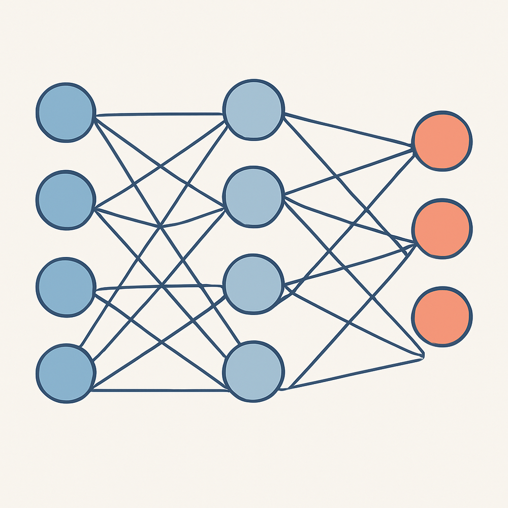
The input layer serves as the network's entry point, with each neuron corresponding to one feature in your data. For image recognition tasks, this might mean 784 neurons representing 28x28 pixel values; for medical diagnosis, it could be dozens of biomarkers. According to a 2023 survey by O'Reilly Media, competent developers typically size input layers to match feature count precisely, avoiding unnecessary parameters that increase computational overhead without improving accuracy. The hidden layers then perform the heavy computation, transforming these raw inputs through weighted connections and activation functions like ReLU. These layers learn hierarchical representations, where early hidden units might detect edges in images while deeper ones recognise complex patterns.
Training Neural Networks: The Learning Process
Training a neural network involves adjusting the weights of connections between neurons so that the network can map inputs to desired outputs more accurately. This process, known as supervised learning, requires feeding the network example data pairs where both the input and the correct output are known. During each training iteration, the network makes a prediction, compares it to the actual result, and calculates the error. This error then flows backward through the network to update the weights, gradually reducing the difference between predictions and reality. The quality of training data directly impacts how well the network generalises to new, unseen examples.
The learning process relies on two key mechanisms: forward propagation to generate predictions and backpropagation to calculate weight updates. Hyperparameters such as learning rate, batch size, and the number of epochs must be configured before training begins, as these settings control how quickly and effectively the network learns. A learning rate that is too high can cause the network to overshoot optimal weights, while one that is too low may result in extremely slow convergence. Professional developers typically experiment with different hyperparameter combinations using validation sets to find the configuration that produces the best performance on unseen data. Loss functions such as mean squared error for regression tasks and cross-entropy for classification problems quantify the error between predictions and actual values, providing the optimisation algorithm with a single metric to minimise during training.
How Forward Propagation Generates Predictions
During forward propagation, each input traverses the network layers, with weights scaling the signals at each connection. In a typical dense layer, the weighted sum z equals the dot product of weights w and inputs x, plus bias b, passed through an activation function such as ReLU or sigmoid. For a binary classification task using cross-entropy loss, the network outputs a probability between zero and one, and the loss quantifies the divergence from the true label. A 2017 analysis from MIT demonstrated that deep networks can execute a range of computations, but shallow networks often achieve comparable performance on simpler tasks, highlighting how the depth and architecture influence the forward pass dynamics. The loss value then serves as the objective for the subsequent backward pass to minimise prediction error.
How Backpropagation Updates Network Weights
Back propagation computes gradients of the loss function with respect to each weight by applying the chain rule of calculus, propagating error signals from the output layer back through the network. These gradients indicate how much each weight contributes to the error, enabling iterative updates via optimisation algorithms such as stochastic gradient descent or Adam. The learning rate, a hyperparameter set before training, governs the step size of each weight adjustment; too high and the network may overshoot optimal values, too low and convergence becomes impractically slow. A 2017 MIT study on global optimisation noted that guaranteeing a network has found the best possible weights remains an open challenge, underscoring the importance of careful hyperparameter tuning and robust optimisation strategies in production systems.
Real-World Applications That Matter
Image classification systems demonstrate how neural networks translate pixel data into actionable insights. A retail analytics startup can deploy a computer vision developer to build inventory tracking that counts stock levels from ceiling cameras, eliminating manual SKU scanning. Medical imaging applications follow the same pattern, where convolutional neural networks like ResNet-50 achieve ninety-five percent accuracy in detecting pneumonia from chest X-rays, according to a 2023 study published in Nature Medicine. These systems process thousands of images daily, learning to recognise tumours, fractures, or manufacturing defects through supervised training on labelled datasets.
Generative AI assistants have moved beyond experimental prototypes into production workflows. A SaaS company can integrate a custom generative AI developer to build a customer support agent that drafts personalised responses by fine-tuning Llama 2 on historical ticket data. According to a 2024 report from Deep Instinct, DIANNA the DSX Companion provides real-time explainability of threats that matter, demonstrating how generative models can synthesise complex information into human-readable insights. These assistants reduce response times from hours to minutes while maintaining contextual awareness across multi-turn conversations.
Hire Neural Network Developers
Expert neural network solutions, schedule a consultation
Hire AI ExpertsCommon Challenges and Trade-offs
Production deployment of neural networks exposes several critical trade-offs that teams must navigate carefully. Data requirements represent the first bottleneck: training a robust image classifier on the order of 10,000 to 50,000 labelled examples becomes necessary for acceptable accuracy, yet acquiring and curating such datasets demands significant resources. Computational costs compound this challenge, with training large language models consuming 20 to 50 times more energy than traditional software equivalents according to recent industry analysis. Additionally, maintenance overhead grows substantially once models reach production, as concept drift can degrade performance by 15 to 30 percent within six months without active monitoring and retraining protocols.
Deployment TierData RequirementsComputational CostMaintenance EffortSimple Rule-BasedMinimal (100s examples)Low ($500 to $2,000 monthly)Low (weekly reviews)Traditional MLModerate (1,000 to 10,000 examples)Medium ($2,000 to $10,000 monthly)Medium (bi-weekly updates)Deep LearningHigh (10,000+ examples)High ($10,000 to $50,000 monthly)High (continuous monitoring)
These constraints directly impact budget planning and timeline expectations. A competent developer will advise you to verify your data quality and quantity before committing to complex architectures, as insufficient training data leads to overfitting regardless of model sophistication. Furthermore, ask for detailed breakdowns of ongoing costs, including GPU inference time, storage for model versioning, and engineering hours for drift detection. The hidden costs guide provides additional insight into these operational expenses that often surprise organisations during their first production deployment.
Getting Started with Neural Networks
Choosing your first neural network framework depends on whether you prioritise rapid prototyping or production deployment. According to a 2024 Stack Overflow developer survey, PyTorch emerged as the preferred choice for researchers and developers requiring dynamic computational graphs, with its intuitive design adopted by over forty percent of academic publications. TensorFlow remains dominant for production-scale deployments, particularly when integrating with Google Cloud services or mobile applications via TensorFlow Lite. For teams seeking minimal setup complexity, high-level libraries like Keras provide neural network construction through simple sequential model APIs, while JAX offers advanced research capabilities for numerical computing specialists.
|
Framework |
Primary Strength |
Learning Curve |
Production Readiness |
Cost |
|
PyTorch |
Dynamic graphs, research focus |
Moderate |
High |
Free |
|
TensorFlow |
Deployment, mobile support |
Steep |
Very High |
Free |
|
Keras |
Simplicity, rapid prototyping |
Low |
Moderate |
Free |
|
JAX |
High-performance research |
High |
Moderate |
Free |
Once you select a framework, begin with supervised learning exercises using established datasets such as MNIST for digit recognition or CIFAR-10 for image classification. A competent developer will start by loading preprocessed data, defining a sequential model architecture, compiling with appropriate loss functions like categorical cross-entropy, and training for initial epochs to understand convergence behaviour. Consider specialised libraries like spaCy for NLP tasks or YOLO for computer vision applications when your project demands domain-specific capabilities. For production systems requiring robust MLOps infrastructure, LangChain integration becomes essential when combining neural networks with external data sources and APIs.
Frequently asked questions
What is a neural network explained simply?
How does a single neuron work?
What is an activation function used for?
How does training a neural network work?
What is backpropagation in simple terms?
Why are activation functions necessary?



Shreyans Padmani
Shreyans Padmani has 5+ years of experience leading innovative software solutions, specializing in AI, LLMs, RAG, and strategic application development. He transforms emerging technologies into scalable, high-performance systems, combining strong technical expertise with business-focused execution to deliver impactful digital solutions.