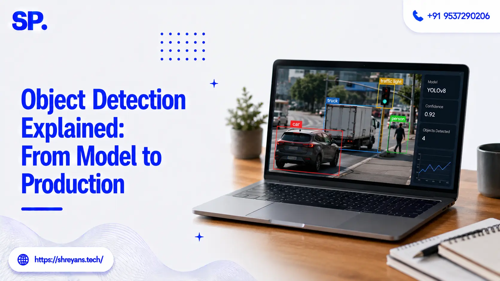
Object Detection Explained: From Model to Production

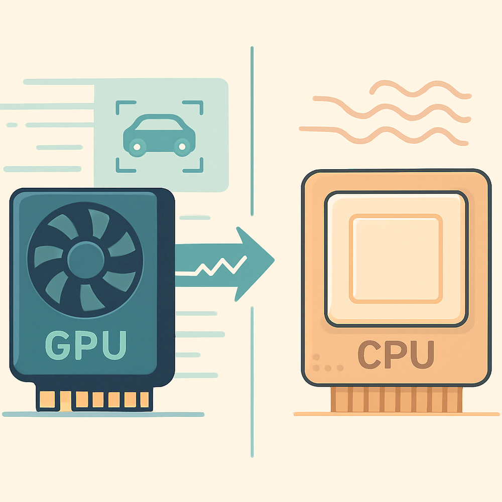
A current-generation detector scores 53.1 mAP on COCO and runs inference in 4.7 milliseconds on a T4 GPU with TensorRT. The same model on a CPU takes roughly 220 milliseconds — about 47 times slower, on hardware plenty of deployments actually use.

Researchers have a name for this: the export gap, the discrepancy between performance observed during GPU training and latency realised on deployed hardware. Training a detector has never been easier. Closing that gap is where most projects stall, and it shapes every decision below. This piece sits within the broader computer vision for business picture.

Classification answers "what is in this image?" with a single label. Object detection answers "what is here, and where?", returning for each object a bounding box, a class label, and a confidence score. Segmentation goes further again, producing a pixel-level mask instead of a box.

That middle option, location plus identity plus confidence, covers a wide range of commercial object detection use cases:

The common thread is that position carries the business meaning. Knowing a defect exists is useful; knowing it sits on the weld seam is actionable. computer vision in manufacturing covers how that plays out across production and quality workflows.

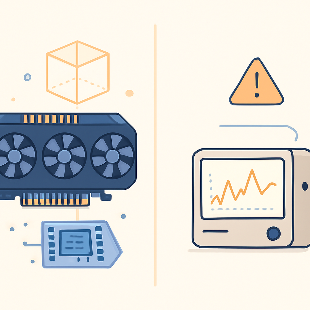
Model benchmarks are published under conditions that rarely match deployment: a server-grade GPU, full floating-point precision, batched inputs, and a curated dataset. Production is usually the opposite, an edge device, reduced precision, one frame at a time, and imagery from your camera rather than COCO.

The gap this opens is not a rounding error. Benchmarking across edge platforms found CPU-only execution of large detectors on a Raspberry Pi 5 produces multi-second per-frame latency, which is simply not viable for real-time work, while the same architecture on a Jetson Orin NX with TensorRT runs comfortably. The model didn't change. The runtime did.

The practical consequence is that choosing a model on mAP alone is choosing on the least deployment-relevant number available.

A working deployment moves through four steps, and the middle two are where most of the engineering time actually goes.

Export cleanliness is worth weighting heavily at model selection time. An architecture that converts without custom operators or unsupported layers reaches production in days; one that needs bespoke kernels for every target runtime can consume weeks. This is precisely why recent detector designs have traded small amounts of benchmark accuracy for simpler graphs that export cleanly across runtimes.

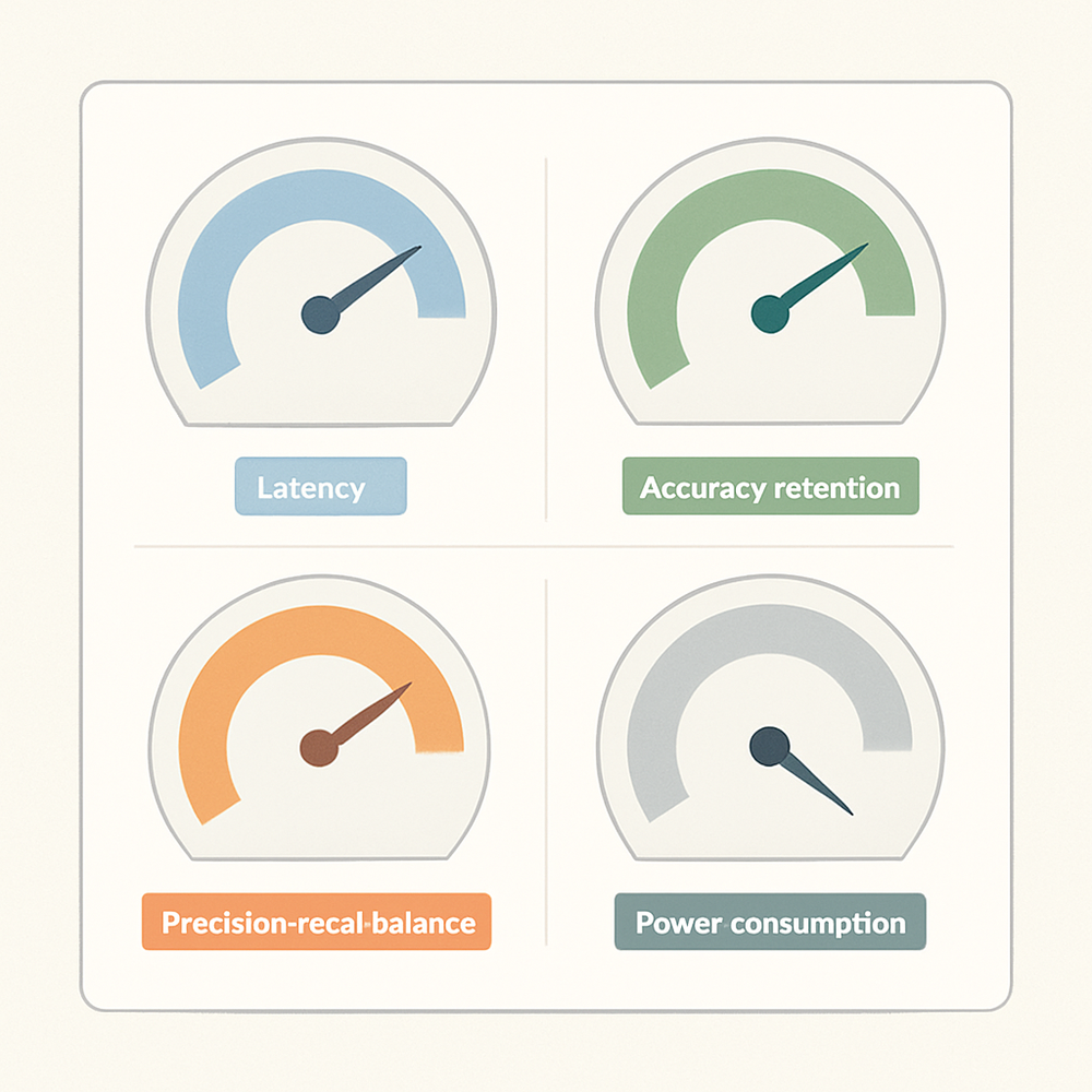
Four numbers predict deployment success better than benchmark accuracy does.

Latency at the 95th percentile on your target hardware, not the average on a T4. Accuracy retention after export and quantization, measured on your own held-out images rather than COCO. Precision and recall at your chosen confidence threshold, since the threshold is a business decision about the relative cost of a miss versus a false alarm. And power draw, if the device is battery-powered or thermally constrained.

A vendor or contractor who reports only mAP is describing the easy part of the problem. vetting a CV consultant covers the wider set of questions worth asking before an engagement starts.